Critic-Oriented Bimanual Badminton Receive in Simulation

Goal: get a stationary bimanual arm to return a badminton serve with either hand, in simulation. The result is one single-arm network that drives both arms, and a small critic model to pick either the left or right arm. On 8192 serves it has never seen, it hits 97.9%, splits the work 49/51 between the arms, and sends 94% of returns over the net.

Simulation setup

The robot is WATonomous' Pioneer bimanual arm with 6 degrees of freedom per arm (normally 7 except both grippers are always shut). The shuttle is a point mass under quadratic drag set to 6.75 m/s terminal velocity. The racket is a simple rigid body with a calibrated contact model, tuned such that the shuttlecock rebounds with ~70% efficiency.

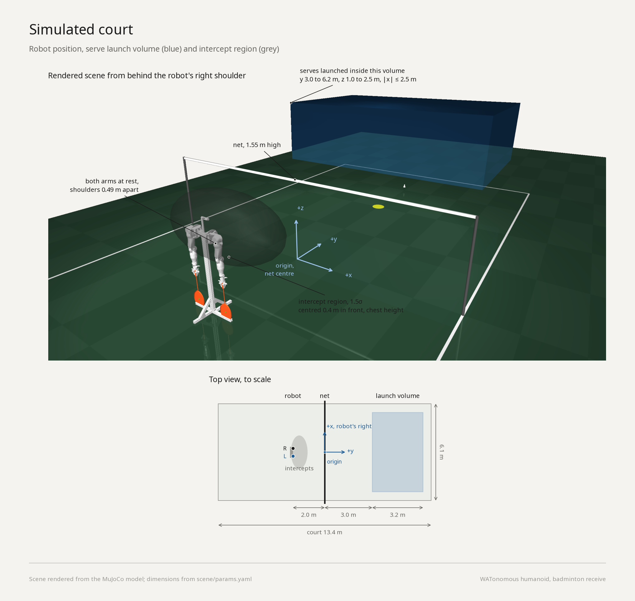Figure 1: Simulated court. Rendered scene with the launch volume and intercept region, and the top view to scale.

The net is at $y = 0$ and the stand is centred on the court 2 m behind it, so the two shoulders sit at $x = \pm 0.245$ m. Serves are launched from a box 3.0 to 6.2 m past the net, 1.0 to 2.5 m high and up to 2.5 m either side, and arrive 0.9 to 1.4 s later in a region centred 0.4 m in front of the robot at about chest height, 4 to 8 m/s and 20° to 60° below horizontal.

Serves come from a bank of 4096 shots sampled from that distribution. Training draws from one bank. Every figure and number in this post is from a separate evaluation bank: 4096 serves sampled with a different seed, none of which appeared in training, run for 8192 episodes. The two banks give the same numbers, so the policy is not memorising serves:

	training bank	evaluation bank
serves hit	98.2%	97.9%
right / left arm	50 / 50	49 / 51
returns clear the net	94.3%	94.3%
median landing error	1.04 m	1.00 m

The same bank moves by up to 0.3 points between reruns (the filter noise and the arm draw differ each time, and the GPU model changes the numerics), so the gap is inside that noise.

MuJoCo was selected as the simulation environment over Isaac Lab for two main reasons: CPU MuJoCo allows for rapid local iteration without a GPU and Isaac Lab's advantages (rendering, sensor simulation) are not advantageous in this use-case. Training runs on MuJoCo Warp through mjlab, 1024 environments at a time, with rsl_rl's PPO.

Policy inputs and outputs

The policy is a plain MLP, $61 \to 512 \to 256 \to 128 \to 6$ with ELU between layers. Inputs are normalised by running statistics. In training the outputs are the mean of a Gaussian with one learned standard deviation that PPO samples from. At deployment the mean is used directly. The network has no hidden state. The only memory in the loop is the previous action fed back as an input and the filter's own recursive estimate.

An intentional design decision is that the final policy should never see the true shuttle state. A batched extended Kalman filter tracks the shuttle from noisy position measurements (3 cm per axis at 50 Hz), and the filter's drag-model rollout gives eight future positions at 0.1 s spacing as a trajectory prior. The policy's input at each 50 Hz tick is

$$o_t = \big[\, q,\ \dot q,\ p_f,\ n_f,\ a_{t-1},\ \hat p,\ \hat v,\ \tau,\ \sigma \,\big] \in \mathbb{R}^{61}$$

where $q, \dot q \in \mathbb{R}^6$ are the active arm's joint positions and velocities, $p_f, n_f \in \mathbb{R}^3$ are the racket face centre and its outward normal, $a_{t-1} \in \mathbb{R}^6$ is the previous action, $\hat p, \hat v \in \mathbb{R}^3$ are the EKF's shuttle position and velocity, $\tau \in \mathbb{R}^{8 \times 3}$ is the trajectory prior (the EKF state rolled forward through the drag model to eight points 0.1 s apart), and $\sigma \in \mathbb{R}^7$ is the EKF's standard deviation on $(\hat p, \hat v)$ plus one scalar for how far the prior jumped since the last tick, so the policy can tell a settling estimate from a converged one.

The output is

$$a_t \in \mathbb{R}^6,$$

a joint position target per motor of the active arm. It is mirrored for the left arm, then rate-limited and low-passed exactly as joint_command does on the hardware before the PD actuators see it.

There is no bimanual network. The policy is a single-arm policy. The inputs and outputs are mirrored for the left arm so that the policy only needs to solve the right arm receive. Every observation is expressed in the active arm's frame. For the right arm, the world is shifted so the arm's swing plane is $x = 0$. For the left arm, the world is first mirrored about the body's centre plane ($x$ becomes $-x$, joint angles negated) and then shifted the same way. The left arm sees exactly what the right arm would see in the mirrored shot, so both arms run the same weights and the pair is symmetric by construction. Which arm is active is decided by a separate network, described in Arm selection.

The rationale behind simulating an EKF rather than just giving raw positions as input is that a policy that sees raw positions would have to learn shuttle aerodynamics implicitly. However, simulated aerodynamics are not the same as real-world aerodynamics. If the policy assumes the simulation's quirks, it will not transfer well to the real arm. Instead, we use an EKF as a model of our real-world perception pipeline, so a policy that learns to use it should transfer better, assuming that our real birdie estimation is generally accurate.

Arm selection

The policy does not select which arm to use. Instead, choosing an arm is done by the critic, a network PPO trains anyway and normally throws away.

PPO trains two networks side by side. The actor is the policy above, $\pi: o_t \mapsto a_t$. The critic is a value function

$$V\colon o_t \mapsto \mathbb{R},$$

an MLP of the same shape, $61 \to 512 \to 256 \to 128 \to 1$, that takes the same observation and outputs one number: its estimate of the total reward the actor will collect from this state onward. Its only job in training is to tell the actor whether each step went better or worse than expected. Once training ends it has no further use, and it is not part of a deployed policy.

Here it is kept, because it already answers the question we need: how well will this arm do from this state? Nothing new is trained for the choice; the critic is reused as a scorer and the arm with the higher score takes the shot.

Because the observation is built in the active arm's frame, the critic's number is specific to an arm. $V(o_t)$ gives "how well does this arm do if it takes the shot from here". During training the active arm is drawn 50/50 at reset and holds the start pose for a random delay of up to 0.2 s before it may move. The critic thus learns that value for both arms, from both early and late starts, including serves the chosen arm cannot reach.

At deployment both arms wait at rest. Each tick the chooser builds the observation twice, once in each arm's frame, and evaluates the critic on both:

$$\Delta_t = V(o_t^{\mathrm{R}}) - V(o_t^{\mathrm{L}}).$$

The right arm is locked in as soon as $\Delta_t > m$, the left arm as soon as $\Delta_t < -m$, and if neither has happened by $t = 0.2$ s the arm with the larger value is taken. We use $m = 1.0$. The 0.2 s cap equals the training swing delay: the policy practised starts anywhere in 0 to 0.2 s and nowhere later. The fastest serves also leave little more than that before the swing has to begin.

The chooser critic is not the one the policy was trained with. The policy's own training critic sees the true shuttle state (see Training recipe), which the robot cannot. The chooser is the critic from a second PPO run of the same task, actor and critic both on the 61 robot observations. That run's actor is a sibling policy that is never deployed; its critic is kept. Strictly, the chooser estimates how well the sibling would do from each arm, but the two policies share a start, a reward and a task, and only the difference between the arms matters. Swapping in the teacher's critic, trained with yet another actor, moves the hit rate by under a point.

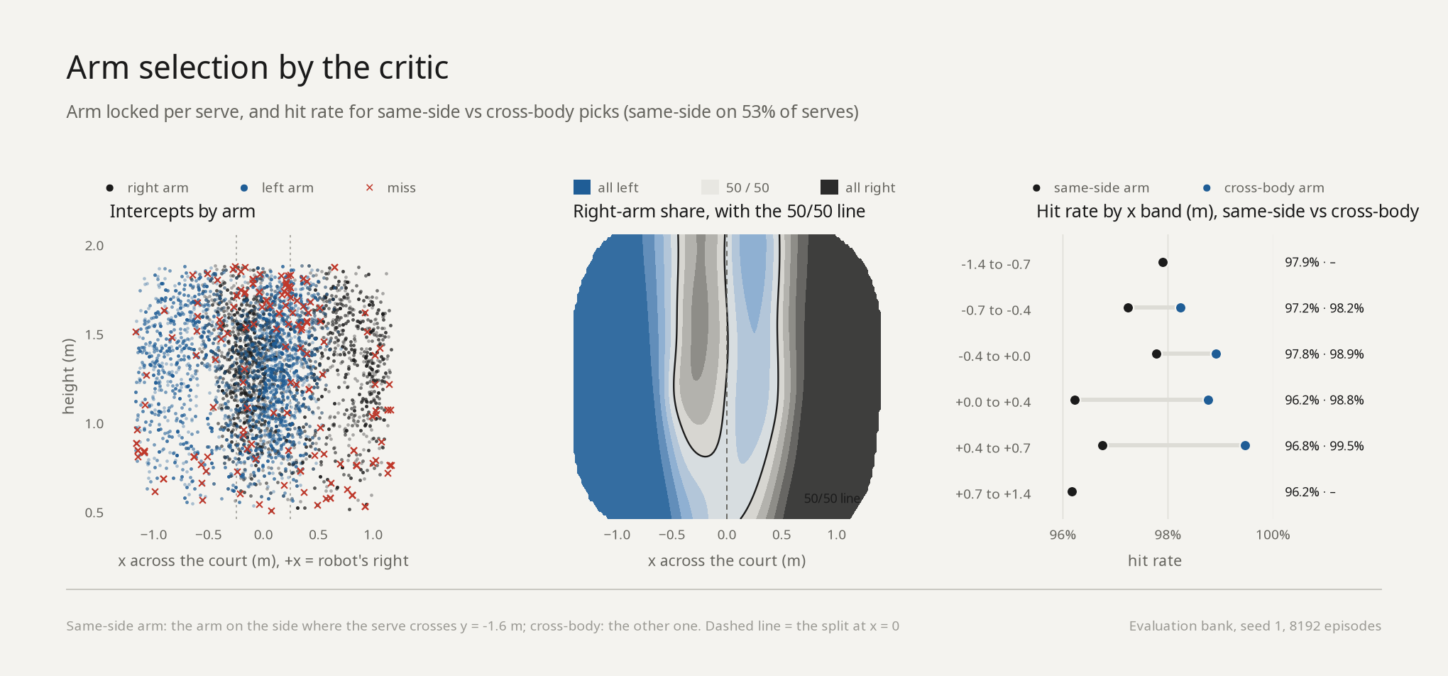Figure 2: Arm selection on the evaluation bank. Every intercept coloured by the arm that took it, the share taken by the right arm with the 50/50 line, and the hit rate for same-side and cross-body picks.

The picks are not what a naive rule would produce. The obvious rule is the same-side arm: serves left of centre go to the left arm. The learned model takes the same-side arm on 89% of serves outside the centre band and on only 28% inside it ($|x| < 0.4$ m), where it prefers the cross-body arm. Over the whole bank, cross-body picks hit 98.8% and same-side picks 97.0%. Whatever the critic is reading in the joint state and the approach angle, it is a better rule than the naive solution.

Most locks happen at the cap. With $m = 0.5$ the median lock is 0.04 s at the same hit rate, and a cap of 0.3 s, outside the training window, drops the hit rate to 85%.

Training recipe

Training consists of four runs, each starting from the previous checkpoint.

1. Teacher. PPO on the privileged observation: true shuttle state, intercept point, time to intercept. 6000 iterations.
2. Distillation. A fresh actor on the 61 robot observations, trained to match the teacher's action on every state it visits (MSE). 1500 iterations.
3. Student PPO, privileged critic. The distilled actor fine-tuned with PPO; the critic sees the privileged observation, the actor does not. 6000 iterations. This actor is deployed.
4. Student PPO, robot critic. Same fine-tune, critic on the robot observations. 6000 iterations. This critic is the chooser.

The active arm is drawn 50/50 at reset and holds the rest pose for a random 0 to 0.2 s before it may move.

setting	teacher	distillation	student PPO
parallel environments	1024	–	–
control rate	50 Hz (20 physics steps of 1 ms per action)	–	–
episode length	3 s	–	–
rollout per iteration	24 actions per environment	–	–
epochs / minibatches	5 / 4	1 / n/a	5 / 4
learning rate	$3 \times 10^{-4}$	$10^{-3}$	$10^{-4}$
entropy coefficient	0.005	n/a	–
initial policy std	0.5	0.1	0.5
iterations	6000	1500	6000 each

Reward

The same reward drives every PPO run. $d$ is a distance in metres, $p^*$ the intercept point, $v$ the shuttle velocity after the hit. rsl_rl multiplies each term by the control period (0.02 s), so a weight of 100 on a one-off event is worth 2.0.

term	paid	value	weight
face contact	once, on the tick the face first meets the cork	1	+100
approach	every tick until the intercept	$\exp(-d^2 / 0.8^2)$, $d$ from the active face to $p^*$	+1
approach, fine	every tick until the intercept	$\exp(-d^2 / 0.15^2)$	+5
return flight	every tick after the hit	$\min\big((v_y + 0.5\,v_z)/6,\ 1\big)$, clamped at 0	+2
return landing	once, at the hit	$\exp(-d^2 / 2 \cdot 1.5^2)$, $d$ from the predicted landing to the serve's origin; 0 if the predicted flight does not clear the net	+100
arm clash	every tick the rackets or forearms touch	1	−50
action rate	every tick	$\lVert a_t - a_{t-1} \rVert^2$	−0.05
joint limits	every tick	distance past the soft joint limits	−5
joint velocity	every tick	$\lVert \dot q \rVert^2$	−0.002

There are two approach terms because one width cannot do both jobs. At $\sigma = 0.8$ m the reward is still non-zero a metre away, so the arm is pulled toward the shuttle from the rest pose, but it is nearly flat in the last 30 cm and cannot tell close from exact. At $\sigma = 0.15$ m it is zero beyond 30 cm and rises steeply in the last 15 cm, so it rewards more exact placement.

The landing term is paid at the hit, not at the landing. On the tick of contact the shuttle's velocity is run forward through the drag model to predict where it will come down, and the reward for that prediction is given immediately, so the swing is credited on the tick it happens rather than two seconds later.

Episodes are terminated when the shuttle touches the floor or the net, when the two arms touch, or at 3 s.

Evaluation results

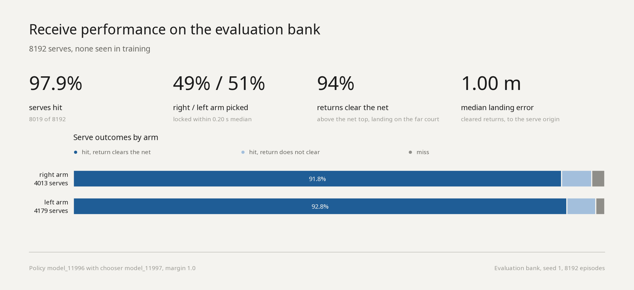Figure 3: Receive performance on the evaluation bank. Headline numbers and the outcome of every serve per arm.

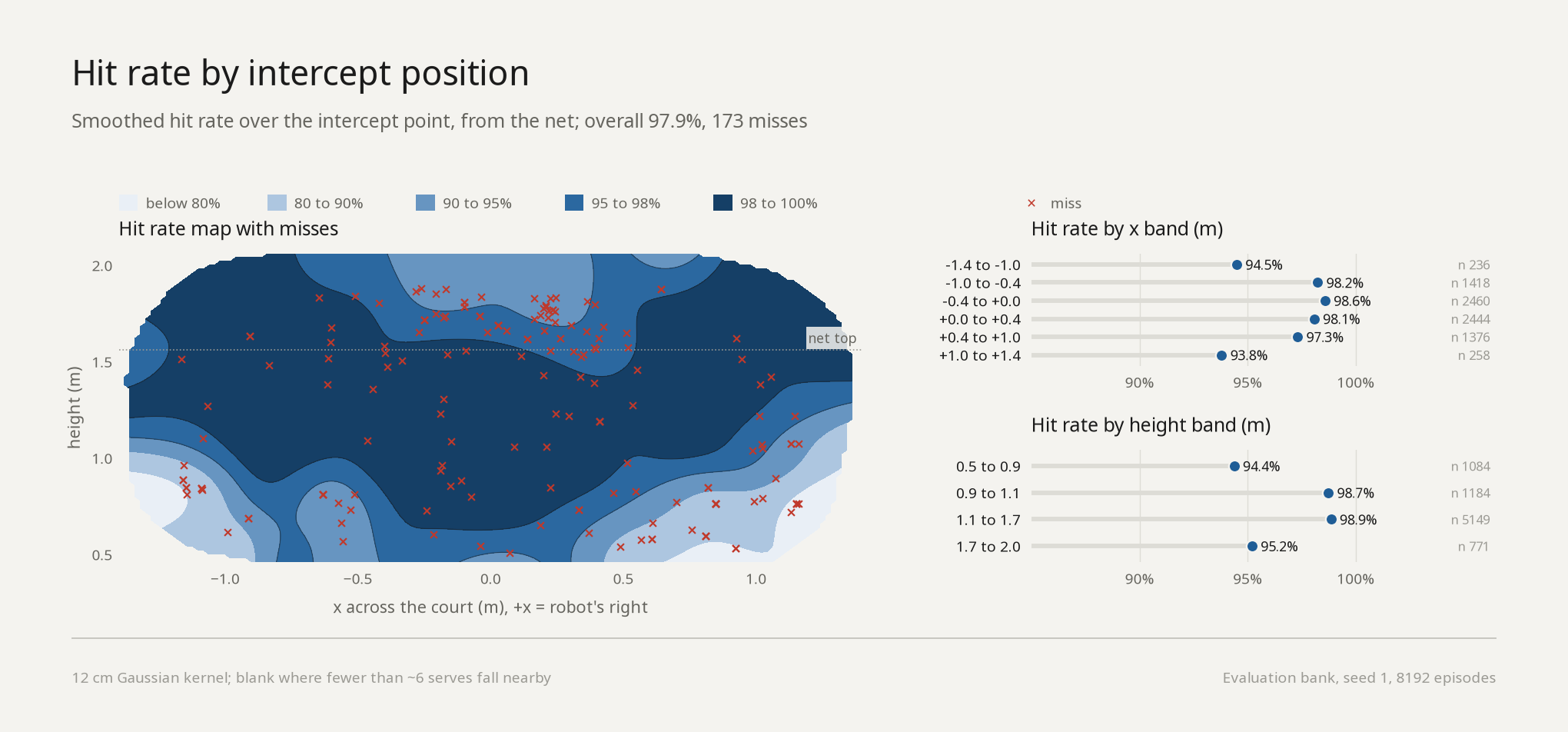Figure 4: Hit rate by intercept position, seen from the net, with the rate per lateral and height band.

173 misses out of 8192. They cluster where you would expect: wide serves beyond $|x| = 1$ m (94% hit), low serves below 0.9 m (94%), and the top of the reach above 1.7 m (95%). Everything within 1 m of centre and between 0.9 and 1.7 m high is hit at 99%.

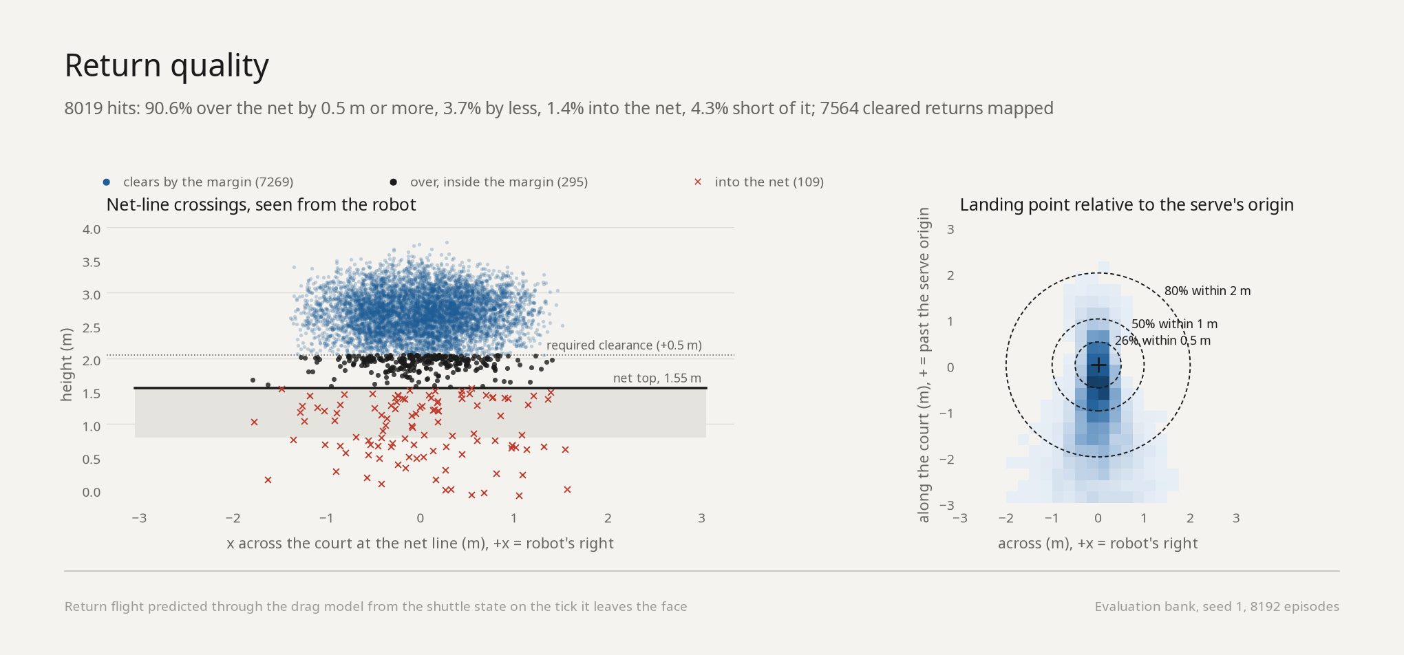Figure 5: Return quality. Where the returns cross the net line, and where they land relative to the serve's origin.

The return is the weaker half. 94% of hits clear the net (91% by the 0.5 m margin), 1% go into the net, and 4% come down on the robot's side. Of the returns that clear, 50% land within 1 m of where the serve was launched from, with a median error of 1.00 m. Aim is the next lever on the reward side.

Open problems

Wrist torque: The wrist motor (GL40) is rated for 0.25 Nm continuous and 0.73 Nm peak. In simulation it is above the continuous rating for about 81% of each swing and hits the peak clamp in about half of all episodes. The shoulder and elbow motors stay below their continuous ratings more than 90% of the time. A real GL40 driven like this would overheat. Options are a lighter racket, a stronger wrist motor, or a thermal limit in the controller, and one of them has to be chosen before the policy runs on hardware.

Perception: The policy consumes a filtered shuttle state and its uncertainty (Policy inputs and outputs), but the perception stack that would produce it does not exist yet. The simulated filter is a guess at what a camera-based tracker will give. If the real tracker is slower, noisier, or loses the shuttle near the net, the policy has only seen the easier version. Building the tracker, measuring its error profile, and retraining with that profile in the simulated filter is most of the remaining work. The output side is simpler: the action targets go through the same joint_command path the hardware already uses.

The code is in the humanoid repo under src/simulation/badminton, and the checked-in models reproduce the numbers above with scripts/eval_rl.py --bank-seed 1.