Fine-tuning π₀.5 for Pick and Place
Goal: get Pioneer's left arm to pick up a cube and place it in a tray in Isaac Sim, from camera images and a text prompt. The approach: fine-tune the π₀.5 vision-language-action (VLA) model on demonstrations recorded with a leader arm, training only the action expert on top of a frozen vision-language backbone.
The policy after 6,000 weight updates, running in Isaac Sim over several attempts in a row. The two smaller windows are what the policy sees: the left wrist camera and the base camera.
Setup
| Parameter | Value |
|---|---|
| Robot | Pioneer bimanual arm rig (left arm) |
| Task prompt | "pick up the cube and place it in the tray" |
| Model | π₀.5 from LeRobot's pi05_base: frozen PaliGemma backbone, trained action expert |
| Data | 71 teleoperated demonstrations, 5,654 frames at 25 fps |
| Cameras | 3 views at 256 × 256: base and both wrists |
| Training | 6,000 updates of 32 samples, AdamW, warmup and cosine decay |
| Compute | One 48 GB cloud GPU, with the backbone frozen |
| Stack | LeRobot, PyTorch, Isaac Sim, Weights & Biases |
Links: Code · Dataset · Checkpoint
How π₀.5 is built
Training a policy from scratch takes far more data than one person can record, so the policy fine-tunes π₀.5, a VLA model from Physical Intelligence, starting from LeRobot's pi05_base weights. It has two parts:
- PaliGemma, a vision-language model (VLM) built on the 2-billion-parameter Gemma language model. It reads the camera images, the text prompt and the arm's joint state.
- The action expert, a much smaller action head with about 300 million parameters. It turns what the VLM understood into motion by flow matching: starting from random noise, it refines a chunk of 50 actions (two seconds at 25 Hz) in 10 steps.
 Figure 1: π₀.5. The frozen PaliGemma VLM reads the cameras, prompt and joint state; the trained action expert refines a noisy 50-step action chunk.
Freezing the backbone
- The PaliGemma backbone is already trained on internet-scale images and text, so it can already read a scene and an instruction. What it has never seen is this arm, these cameras and this task.
- It has far too many parameters to fine-tune on 71 short demonstrations: that would need much more memory and risk damaging what it already knows.
- So the backbone is frozen and only the action head — the part that has to adjust to the task — is fine-tuned.
Recording demonstrations
There was no dataset for this arm, so one was recorded in simulation:
- The Pioneer arm in Isaac Sim is a digital twin of the real one.
- It is driven by a 3D-printed leader arm: seven Feetech STS3215 servos used only as encoders, one per joint and one for the gripper.
- Each leader joint maps directly to the matching simulated joint, so moving the leader by hand moves the robot the same way, with no inverse kinematics.
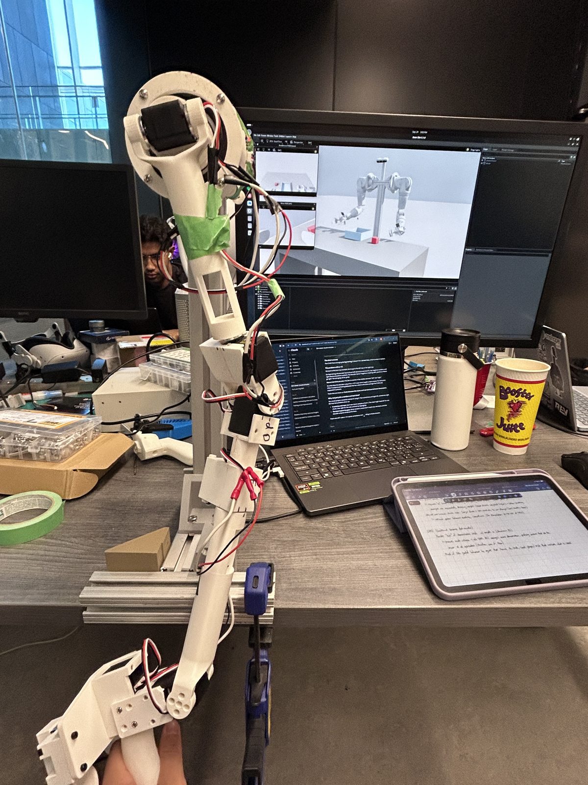
Left: the leader arm — seven servos used as joint encoders, with the scene it drives on the monitor behind it. Right: recording a demonstration; the simulated arm follows the leader joint for joint.
- The recorder saves four things 25 times a second as a LeRobot v3.0 dataset: the arm's joint positions (the state), the leader's joint targets (the action), three camera images and the text prompt.
- The scene (a table, a cube and a tray) has three cameras matched to the real robot's specs: a base camera modelled on an Intel RealSense D455 and one on each wrist. The closer the simulated images are to the real ones, the less the policy has to relearn on the real arm.
- The finished dataset is 71 episodes of about 3 seconds each, 5,654 frames in total.
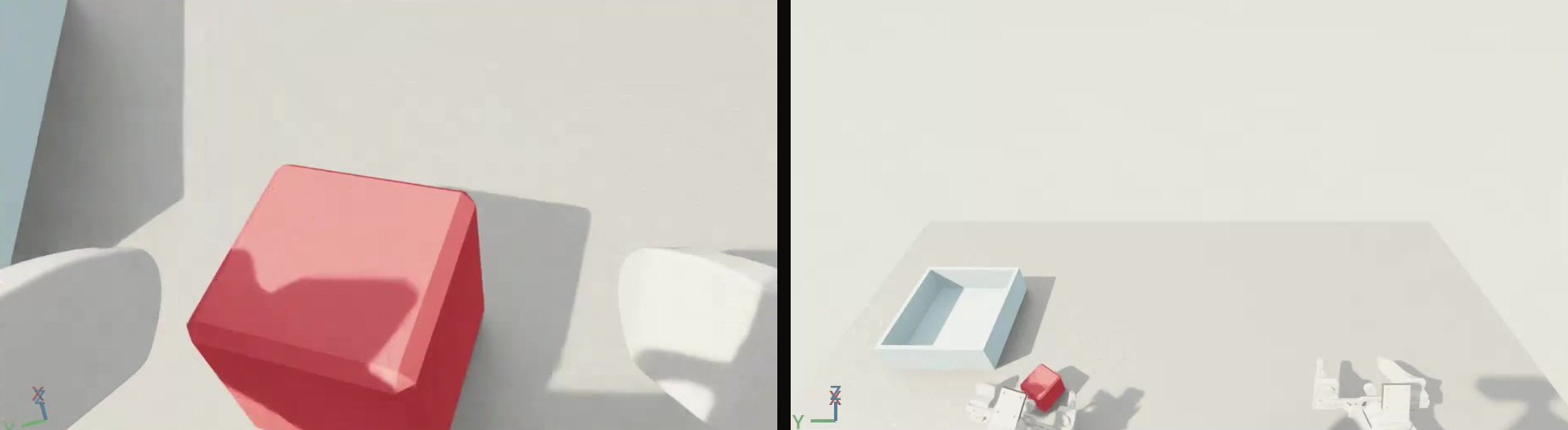 Figure 2: What the policy sees: the left wrist camera, close to the cube, and the base camera looking down at the table.
From a recording to model input
LeRobot's pre-processor and post-processor convert between the dataset and the model:
- Images are resized to 224 × 224, and the prompt and joint state are turned into tokens.
- Joint states and actions are normalized to roughly −1 to 1, using each dimension's 1st and 99th percentile. Without that, a wrist that moves through almost 2 radians would dominate the loss over a gripper finger that moves 0.05 metres.
- The post-processor undoes the normalization, so the output is joint targets in radians again.
- Training uses delta actions: each step the model predicts is an offset from where the arm was when it planned, while the gripper stays absolute. A policy that has not learned much then holds still instead of drifting toward an average pose.
The training script
The training loop is written by hand instead of calling LeRobot's training command. From top to bottom:
| Stage | What it does |
|---|---|
| Setup | Fixes the random seeds, downloads the dataset from the Hugging Face Hub, and checks the Hub and Weights & Biases logins up front, so a missing token fails in seconds, not after hours of training. |
| Model | Loads pi05_base and matches its inputs and outputs to this dataset's cameras and joints. Weights stay in 32-bit floats while the forward pass runs in bfloat16, which is faster and smaller without rounding away small updates. |
| Train / validation split | Holds out one shuffled episode for validation and trains on the other 70. The split is by episode because neighbouring frames are nearly identical. |
| Data loading | Each sample is one frame plus the next 50 actions, shuffled so every update mixes frames from many episodes. |
| Processors | Builds the normalization and tokenization steps from the dataset's statistics, using the delta-action statistics for actions. |
| Freezing | Turns gradients on only for the action expert and its small input and output layers, and gives the optimizer only those parameters. |
| Learning rate | AdamW with a peak of 2.5e-5: linear warmup over the first 100 updates, a hold at the peak, then cosine decay to 10% of the peak over the last 1,000 updates. |
| Training loop | Runs 16 samples per forward pass and adds up the gradients from two passes, so every weight update is based on 32 samples. Gradients are clipped to a norm of 1.0. |
| Validation | Scores the held-out episode every 250 updates with the same random noise each time, so a change in validation loss comes from the weights. |
| Checkpoints and logs | Logs loss, learning rate and gradient norm to a CSV file and to Weights & Biases, and uploads the final 14.5 GB checkpoint to the Hub. |
Making it fit
- π₀.5 ran out of memory on a 12 GB laptop GPU, so training moved to a 48 GB cloud GPU.
- Gradient accumulation keeps the update size independent of the hardware: a batch of 2 over 16 passes on a small GPU and a batch of 16 over 2 passes on the cloud GPU both give 32 samples per update.
- Freezing the backbone saves memory too: it needs no gradients and no optimizer state.
- The first updates of a fine-tune are the riskiest, because the gradients are largest then: the gradient norm starts near 3 and falls to about 0.4 within 60 updates. The warmup keeps those steps small so they cannot wreck the pretrained weights, and the cosine decay lets them settle at the end.
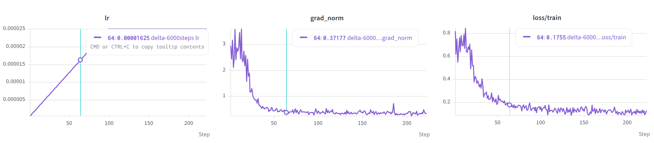 Figure 3: The first 200 updates: the learning rate ramps up while the gradient norm and the training loss fall quickly.
Detaching the frozen backbone
In π₀.5 the VLM and the action expert run side by side through 18 layers, and in each layer they share one attention step so the action tokens can read the image and prompt tokens. Because of that shared step, PyTorch treats every VLM activation as part of the training graph and keeps it in memory for the backward pass, even though the VLM's weights are frozen.
None of that is needed. The attention mask stops the image and prompt tokens from looking at the action tokens, so the VLM's outputs never depend on anything being trained. Wrapping LeRobot's layer function to call .detach() on the VLM's output after every layer leaves the action expert's gradients exactly the same, but PyTorch no longer stores the VLM's activations or backpropagates through the 2B-parameter backbone, which saves a lot of GPU memory.
_compute_layer_complete = pi05_modeling.compute_layer_complete

def _compute_layer_frozen_prefix(*args, **kwargs):
    prefix_out, suffix_out = _compute_layer_complete(*args, **kwargs)
    return [prefix_out.detach(), suffix_out]

pi05_modeling.compute_layer_complete = _compute_layer_frozen_prefix
 Figure 4: The detach trick. The action expert reads the VLM's keys and values in every layer, but the VLM's output is detached, so gradients flow back through the action expert only.
Results
The first run was underfit
- The first cloud run used 1,000 weight updates, about 5.7 passes over the roughly 5,600 training frames. The loss went down, but that says little about whether the arm would do the task.
- An offline evaluation gives the policy recorded camera frames and joint states and compares its predicted actions with what was actually done on the leader arm, next to a baseline that just holds the arm's current position.
- The policy lost to that baseline. Over the first 0.4 seconds of each prediction — the part the arm executes before the policy plans again — its arm-joint error averaged about 10 degrees on episodes it had trained on, against about 5.5 degrees for holding still.
- A policy that is worse than standing still on its own training data has not learned the demonstrations yet, so it needed more training.
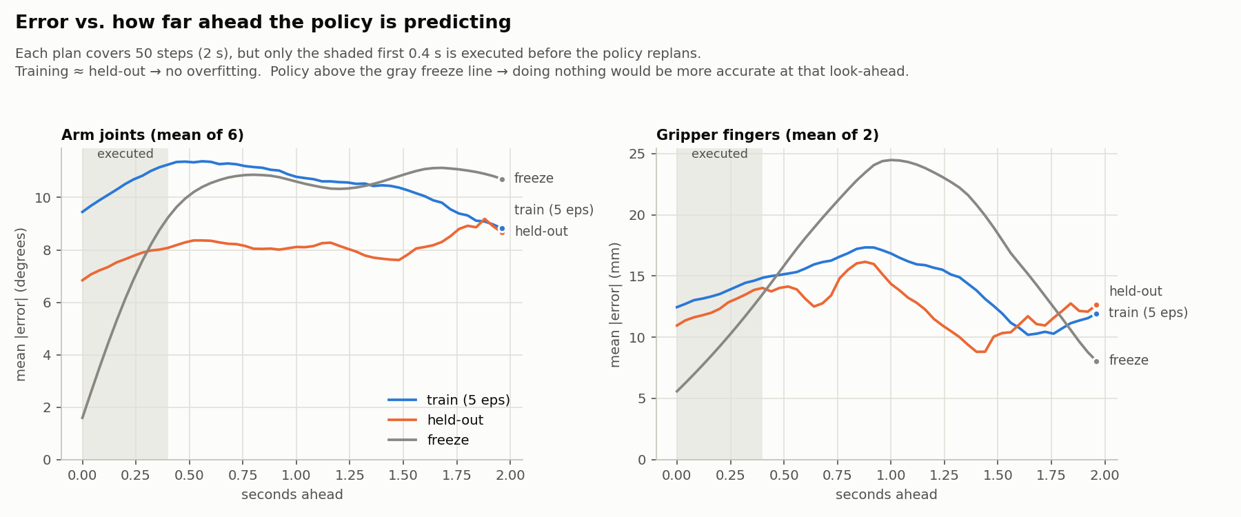 Figure 5: Error against look-ahead, first run. In the shaded 0.4 s that gets executed, the policy (blue and orange) is less accurate than holding still (grey).
Training longer
- The run was raised to 6,000 updates, about 34 passes over the data. The training loss fell from about 0.70 to about 0.013, and in simulation the arm now picks up the cube and places it in the tray, as in the video at the top.
- Validation loss on the held-out episode was lowest between about 750 and 2,000 updates, around 0.07, then climbed to 0.144 while the training loss kept falling: the usual sign of overfitting.
- One held-out episode is a noisy measure, but the trend is steady: the first run trained too little, this one probably too much, and the best checkpoint is likely somewhere in between.
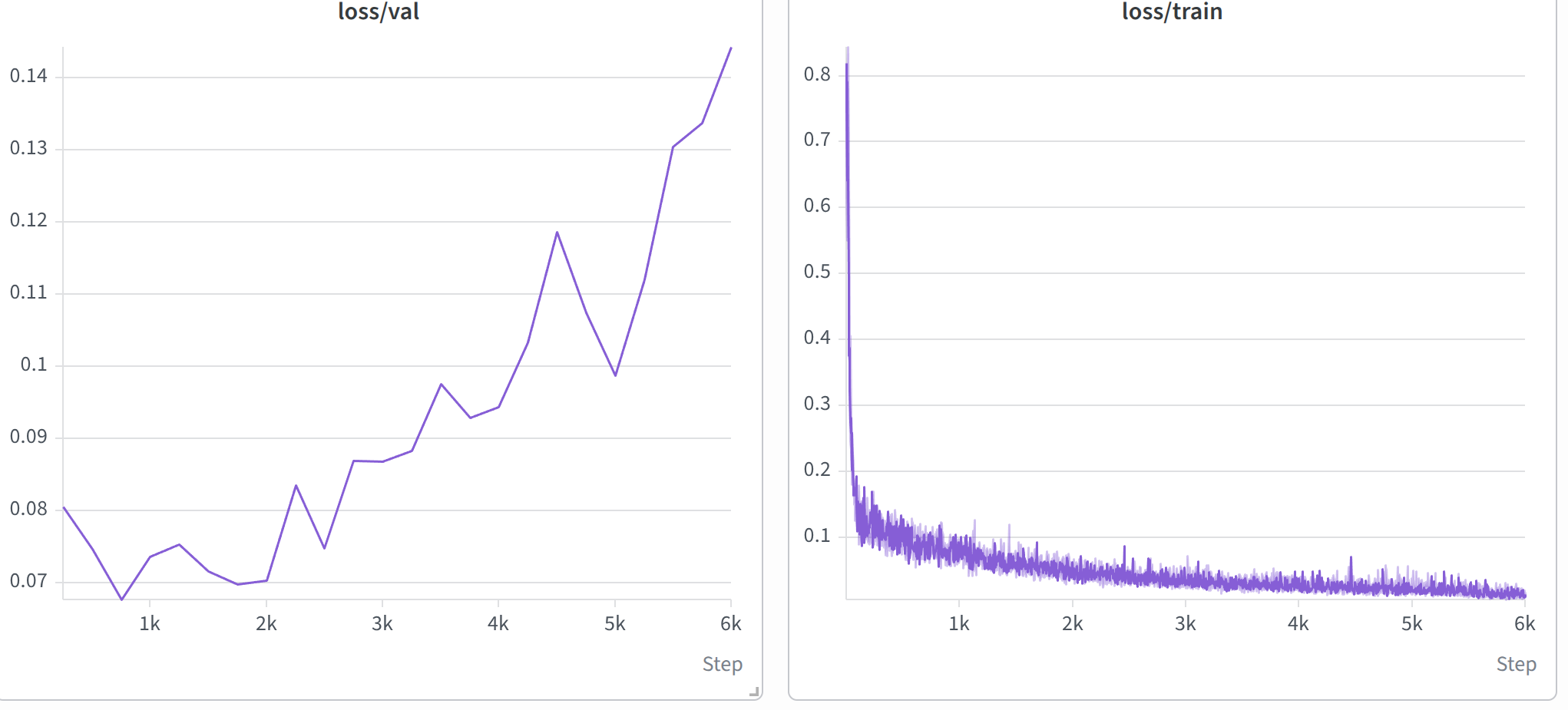 Figure 6: The 6,000-update run. Validation loss (left) bottoms out early and then rises; training loss (right) keeps falling.
:::tip Next steps
- Save checkpoints more often, and pick one by validation loss and success in simulation.
- Record more demonstrations, with more variety in where the cube and tray start.
- Measure a success rate over many resets.
- Try the policy on the real arm.
:::